Designing a Microphone Array to Detect FPV Drones

You can detect an FPV drone before you can see it. The motors and props produce a characteristic harmonic signature — blade-pass fundamental and overtones — that sits squarely in the 300–4000 Hz band. So I wanted to understand: if you built a small array of microphones to detect and classify drones acoustically, what shape should it be?

I spent some time reading the literature and running simulations. This post walks through the physics that constrains the design, compares the standard geometries, and lands on a recommendation. The constraints: 16 microphones, the 300–4000 Hz band, and a multichannel algorithm running on an edge accelerator (Hailo / Jetson) — not necessarily classical beamform-then-detect.

What the research says

Two bodies of work bear on this — how people detect drone audio, and how they shape the array.

Detection algorithms. The field has gone through three generations. Early systems exploited the drone's harmonic comb directly — matched filters and spectral-correlation detectors. Effective in quiet conditions, brittle to wind and varying throttle. Then came feature-engineered ML: MFCCs or spectral statistics fed into an SVM or random forest, reaching around 96.7% binary accuracy with modest compute. Today the mainstream approach is a CNN or CRNN over a Mel/STFT spectrogram, pushing detection above 98% and enabling drone-type recognition (AUDRON).

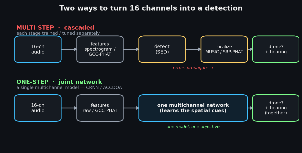
One-step vs multi-step maps to the SELD literature. A cascaded pipeline detects first, then localizes — each stage can be tuned independently, but errors propagate. A joint model does both at once: the CRNN backbone is standard, and the ACCDOA formulation folds detection and DOA into a single regression target. For 16-channel edge inference, a joint CRNN/ACCDOA network fed GCC-PHAT features is the well-supported default — which means the array's job is to give the network rich spatial cues, not to form a textbook beam.

Array topologies. Uniform arrays (ULA, UCA) are the textbook baseline — strong narrowband DOA, but aliasing caps the usable band hard: a 15 cm drone array is unambiguous only to ~1.1 kHz. Aperiodic planar layouts (spiral, GA-optimized) break the grating lobes into a diffuse floor. Sparse / virtual-aperture designs — coprime, nested, fractal — deliberately drop mics off the uniform grid so the gaps between them synthesize a much larger virtual array (a richer co-array) than the mic count alone would suggest; head-to-head benchmarks of these layouts back up how much localization accuracy you can wring from a handful of elements. And 3-D volumetric arrays — tetrahedral, spherical-harmonic MUSIC — give full elevation coverage and remove the up/down ambiguity every flat array has.

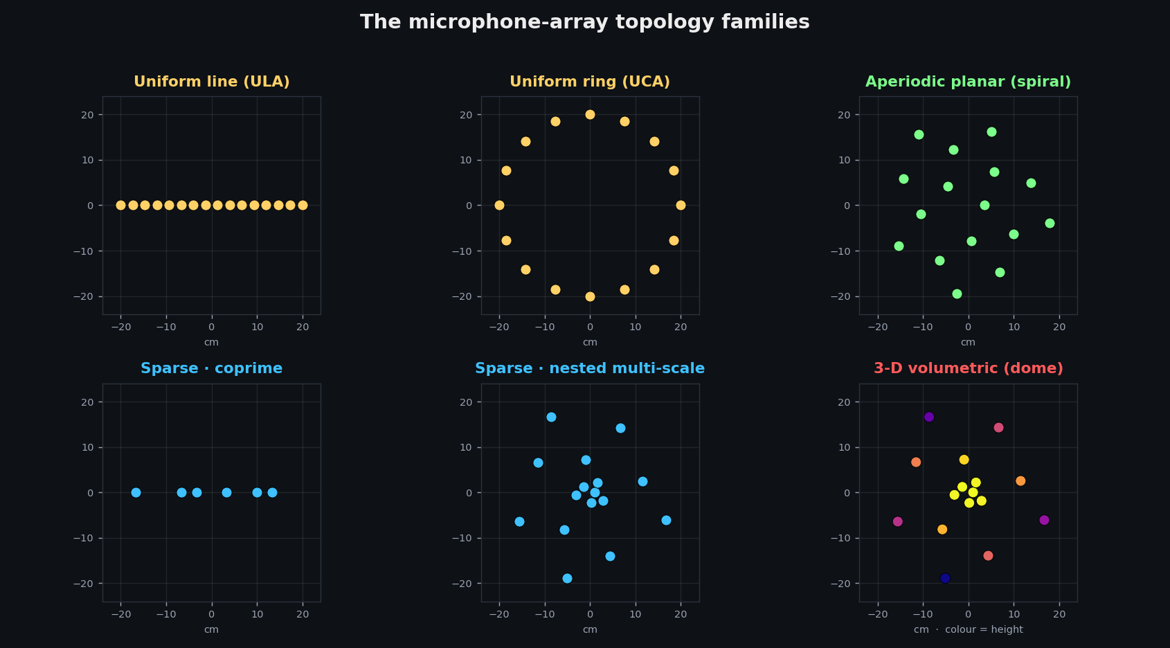
The recommendation below is the drone-tuned intersection of the last two: a sparse, co-array-maximizing layout lifted into 3-D, with the smallest baseline kept ≤4 cm so nothing aliases inside 300–4000 Hz.

The tradeoff that drives everything

Two opposing pressures fight over the spacing between microphones, and with a fixed number of them you can't satisfy both at once.

Too far apart, and directions alias

Arrays localize sound by comparing the phase of a wavefront across microphones. The catch: if the spacing exceeds half a wavelength, two completely different arrival directions produce identical phase samples at every mic — a grating lobe. The array cannot tell them apart.

At 4 kHz the wavelength is 8.6 cm, so to stay unambiguous across the band the smallest spacing must be ≤ 4.3 cm.

Too close together, and resolution is lost

So pack every mic in tight and the aliasing goes away — but now you've thrown away resolution. Angular resolution is set by the array's aperture (its overall span) measured in wavelengths: the main lobe is roughly λ / D wide, so a small aperture smears every direction into one fat blob and two drones a few degrees apart merge into a single blip. This is the diffraction limit — the same reason a bigger telescope mirror sees finer detail. At 300 Hz (λ = 1.14 m) you need a large aperture just to get a usable bearing, which is the exact opposite of packing tight.

The video below sweeps a fixed 16-mic line from tightly packed to widely spread, all at one frequency. Watch the main lobe sharpen as the aperture grows — resolution improving — and then watch phantom copies march in from the edges as the spacing pushes past λ/2, until a false drone sits right among the real directions. That's the whole bind in a single motion:

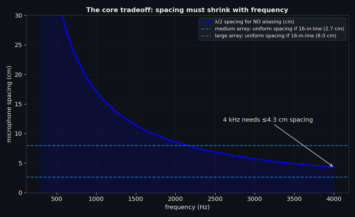
Tight spacing buys an alias-free band; a wide aperture buys resolution; and with only 16 mics a uniform grid can't deliver both — a 1.2 m line at 4.3 cm spacing would need ~28 of them. That irreconcilable pull is what drives the design toward non-uniform, multi-scale layouts: some baselines kept small, others stretched wide.

How geometry shapes the beam

I simulated the far-field delay-and-sum response for the standard candidates: line (ULA), single ring (UCA), spiral, concentric rings, and a hemispherical dome. The most important contrast is uniform vs aperiodic:

A uniform ring grows sharp, discrete grating lobes at high frequency — phantom directions as loud as the real one. An aperiodic spiral with the same mics and same aperture smears that energy into a low, diffuse floor instead. The interactive explorer below lets you sweep frequency and geometry — and steer the look direction — to see this directly:

A beam pattern depends on where you look

There's a subtlety the beam patterns above hide if you only ever steer one way: the response is not a property of the array, it's a property of the array and the look direction. This bites the line array hardest. A ULA only senses the component of the wavefront along its axis, so what it does depends entirely on where the target is relative to that axis.

Steer it endfire (along the line) and the main lobe balloons to ~40° — terrible resolution, because a tilt of the source barely changes the along-axis projection. Steer it broadside (perpendicular) and the lobe sharpens to ~7° — but now there are two of them, a mirror pair at ±90° the array can't tell apart. In full 3-D it's worse than a mirror: a broadside-steered line responds to the entire cone of directions at that angle (drag the explorer to the line array, hit "across (90°)", and orbit it — the lobe is a flat disk). A 2-D array has no privileged axis, so its beam stays essentially the same wherever you steer it:

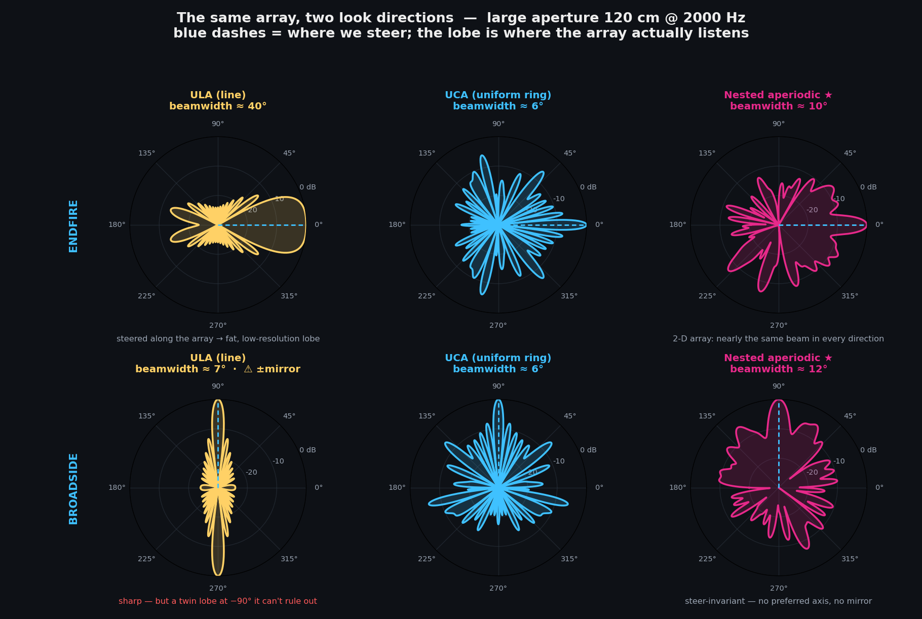
This is the other half of the case against the line array for drone work: even ignoring aliasing, its performance swings wildly with bearing, and a drone can come from any direction. The 2-D and 3-D layouts are the ones you can actually trust to behave the same all around.

The co-array: why geometry matters for a neural network

Every mic pair is one spatial measurement. With 16 mics that's 120 pairs — but on a uniform ring, those 120 pairs share only 8 distinct baseline lengths (15× redundant). An aperiodic layout spreads them across ~100.

In the video the uniform ring collapses its 120 pairs onto just 8 distinct baseline lengths (15× redundant), while the aperiodic spiral spreads them across ~100. That spread is exactly the spatial information a 16-channel network feeds on.

Collapsing that cloud onto a 1-D histogram of baseline lengths makes the trade-offs even sharper — here for the 1.2 m arrays:

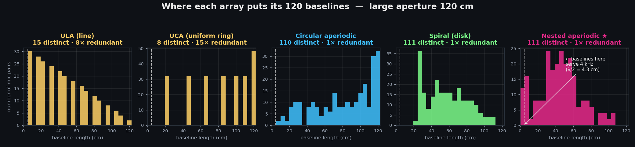
The uniform ring dumps all 120 pairs onto 8 lengths (tall spikes, nothing below ~23 cm). A circular aperiodic ring spreads them richly but still has almost nothing small — which is exactly why its high-frequency sidelobe floor rises. Only the nested array shows the multi-scale signature: a cluster of tiny baselines left of the 4.3 cm line plus a spread out to the full aperture.

More distinct baselines means more independent spatial features, which means easier detection and coarse bearing — without needing classical beamforming at all. Discrete grating lobes are genuine ambiguities a network can't undo from a single snapshot. An aperiodic sidelobe floor is benign and learnable.

The recommendation: a nested-aperiodic dome

A shallow dome carrying a tight central cluster of ~6 mics within a ≤4 cm radius (alias-free cues to 4 kHz) plus ~10 outrigger mics spread aperiodically to the full aperture (low-frequency resolution and SNR), with the centre mics raised out of plane to break the up/down elevation ambiguity that overhead FPV threats create.

Here's the backing comparison (the dome is shown dashed because it shares the nested-aperiodic layout in the horizontal plane — its real advantage is elevation, which an azimuth cut doesn't show):

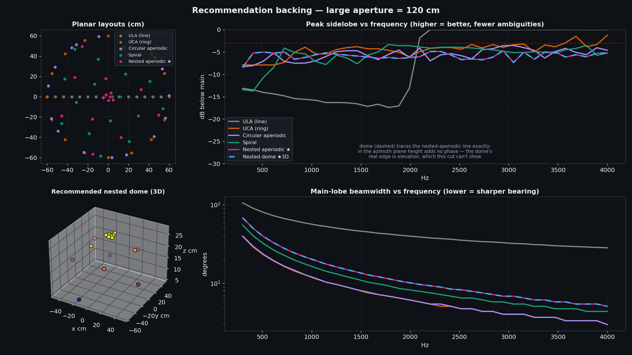
	Medium (~35–40 cm)	Large (~1.0–1.2 m)
Min spacing / alias-free	~2–4 cm / ~7.5 kHz	~3–4 cm / ~4.5 kHz
Beamwidth @ 3 kHz	~20°	~7°
Best for	portability, coarse bearing	long-range, sharp low-freq bearing

If the array has to be flat, drop the dome to a plane. You keep every broadband and diversity benefit and only lose elevation discrimination. The nested-aperiodic disk is the pragmatic default when a 3-D structure isn't practical.

What to avoid: the plain uniform ring (UCA) aliases over most of the band with 16 mics. Popular in the narrowband DOA literature — wrong choice here.

A few practical notes

You don't need beamform-then-detect. A joint CRNN/ACCDOA network fed raw 16-channel input or a GCC-PHAT cross-correlation stack (120 pairs — trivial for a Jetson) handles everything in one pass and maps cleanly to INT8 inference on Hailo or Jetson. Sample at ≥10–16 kHz; 16 ch × 16 kHz × 16-bit is ~4 Mbit/s. Calibrate the measured mic positions carefully — aperiodic arrays depend on it. And MEMS mics (digital I²S/PDM, phase-matched) are the obvious building block: cheap and easy to place on a PCB dome or disk.

The whole simulation — the geometry library, response-curve plots, and the animations above — is a few hundred lines of Python, and it's all on GitHub. The physics is old; the new part is realizing that when a 16-channel network is doing the detection, the right objective isn't a clean beam — it's baseline diversity.